xopto.pf.mienormal module¶

class MieNormal(center: float, sigma: float, nsphere: float, nmedium: float, wavelength: float, clip: float = 5, nd: int = 100)[source]¶

Bases: xopto.pf.miepd.MiePd

Scattering phase function of Normally distributed (number density) spherical particles:

$p(d) = A e^{\frac{-(d - center)^2}{2\sigma^2}}$

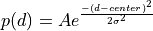
The value of parameter $A$ is computed so as to normalize the integral of the density function on the clipped diameter interval $[center - \sigma clip, center + \sigma clip]$ to 1:

Parameters

center (float) – Distribution/diameter mean (m).
sigma (float) – Distribution/diameter standard deviation (m).
nsphere – Parameters passed to the xopto.pf.miepd.MiePd() base class constructor. See help of xopto.pf.miepd.MiePd class for more details.
nmedium – Parameters passed to the xopto.pf.miepd.MiePd() base class constructor. See help of xopto.pf.miepd.MiePd class for more details.
nd – Parameters passed to the xopto.pf.miepd.MiePd() base class constructor. See help of xopto.pf.miepd.MiePd class for more details.
clip (float) – Distribution/diameter range used to estimate the phase function defined as $[center - clip \sigma, center + clip \sigma]$ .

Examples

Scattering phase functions of Normally distributed microspherical particles with a mean diameter of 1 um and a standard deviation of 100 nm, a mean diameter of 1 um and standard deviation of 50 nm, and a mean diameter of 1 um and a standard deviation of 25 nm compared to a monodisperse 1 um microspherical particles.

>>> from matplotlib import pyplot as pp
>>> import numpy as np
>>>
>>> cos_theta = np.linspace(-1.0, 1.0, 1000)
>>> nmie1 = MieNormal(1e-6, 0.1e-6, nsphere=1.6, nmedium=1.33, wavelength=550e-9, nd=1000)
>>> nmie2 = MieNormal(1e-6, 0.05e-6, nsphere=1.6, nmedium=1.33, wavelength=550e-9, nd=1000)
>>> nmie3 = MieNormal(1e-6, 0.025e-6, nsphere=1.6, nmedium=1.33, wavelength=550e-9, nd=1000)
>>> mmie = Mie(nsphere=1.6, nmedium=1.33, diameter=1e-6, wavelength=550e-9)
>>>
>>> pp.figure()
>>> pp.semilogy(costheta, nmie1(cos_theta), label='Normal(1 um, 100 nm)')
>>> pp.semilogy(costheta, nmie2(cos_theta), label='Normal(1 um, 50 nm)')
>>> pp.semilogy(costheta, nmie3(cos_theta), label='Normal(1 um, 25 nm)')
>>> pp.semilogy(costheta, mmie(cos_theta), label='Monodisperse(1 um)')
>>> pp.legend()
>>>