Reflectance acquired with optical fibers and probes

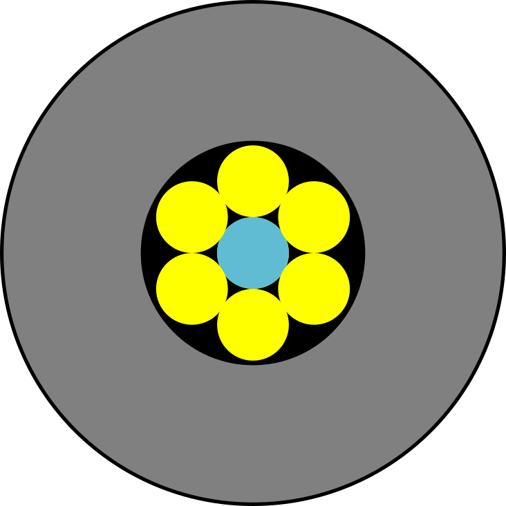
This example (available in examples/mcml/reflectance_optical_probes) shows how to simulate reflectance as acquired with optical fiber probes using four approaches. All approaches utilize a multimode optical fiber source, but different detection schemes. The first detection scheme is a multimode optical fiber situated 220 μm from the center of the source fiber as is commonly the case in a six-around-one optical probe. The second detection scheme utilizes a radial accumulator annular rings which can be integrated over the detector fiber to yield equal reflectance as acquired with the first detection scheme. The third detection scheme utilizes SixAroundOne object which accumulates photon packet weights into seven multimode optical fiber detectors (including the central optical fiber). Finally, the fourth detections scheme is the same as in the third case, however, the top surface model is changed to a realistic case which mimicks the layout of the materials comprising the tip of the six-around-one optical fiber probe, i.e., epoxy filling and stainless steel as shown in the image below.

Importing the required modules and submodules

The required modules and submodules used in this example are listed below. The submodule xopto.mcml.mc can be conveniently used as an interface to the neccessary submodules for sources, detectors, layers, simulators, etc. The submodule xopto.mcml.mcutil.fiber enables utilization of multimode optical fibers, while the submodule xopto.mcml.mcutil.axis enables straightforward definitions of axes objects that are important as input parameters to photon packet accumulators. The submodule xopto.util.convolve holds a helper function for integration of radial annular accumulators to reflectance as acquired through a specified optical fiber probe. Finally, the submodule xopto.cl.clinfo provides functions for working with OpenCL resources, i.e., available computational devices (CPUs, GPUs, etc.). Finally, the standard numpy module provides mathematical functions used in this example.

from xopto.mcml import mc
from xopto.mcml.mcutil import fiber
from xopto.util import convolve
from xopto.cl import clinfo

import numpy as np

Computational device

Select the desired OpenCL computational device (see also OpenCL devices).

cl_device = clinfo.gpu(platform='nvidia')

Note

In this example we have selected the first computational device listed under the Nvidia platform. The string should be changed according to the installed hardware devices.

The layer stack

In this example we use a single-layered turbid medium of 1 cm thickness. The refractive index of the single layer was set to 1.33, while the surrounding medium refractive index is set to 1.45, which corresponds to a uniform boundary with an optical fiber core. The absorption is set to zero, while the scattering coefficient of the single layer is set to 100 1/cm. Finally, the Henyey-Greenstein phase function is utilized with anisotropy factor of 0.8 in the single layer turbid medium. Note that each layer is defined using an instance of Layer, which are then packet into a list and passed to the Layers constructor. The order of the layers is ascending along the positive z axis, which points into the medium. In all cases the top and bottom layers must be provided and correspond to the medium surrounding the single-layer specified in the middle.

d = 1e-2
layers = mc.mclayer.Layers([
    mc.mclayer.Layer(d=0.0, n=1.45, mua=0.0, mus=0.0, pf=mc.mcpf.Hg(0.0)),
    mc.mclayer.Layer(d=d, n=1.33, mua=0.0, mus=100e2, pf=mc.mcpf.Hg(0.8)),
    mc.mclayer.Layer(d=0.0, n=1.45, mua=0.0, mus=0.0, pf=mc.mcpf.Hg(0.0)),
])

Note

All quantities MUST be provided in appropriate units, i.e., distances in m, absorption and scattering coefficients in 1/m.

Source

The multimode optical fiber source is defined using the class MultimodeFiber with a core diameter dcore of 200 μm, combined diameter of core and cladding dcladding of 220 μm, core refractive index ncore of 1.45 and numerical aperture na of 0.22. The multimode optical fiber source is centered at the origin and positioned normally to the turbid medium as noted by the direction and position keyword arguments passed to the UniformFiber source constructor. Note that these are the default values of direction and position.

source = mc.mcsource.UniformFiber(
    fiber=fiber.MultimodeFiber(
        dcore=200e-6, dcladding=220e-6, ncore=1.45, na=0.22
    ),
    direction=(0.0, 0.0, 1.0),
    position=(0.0, 0.0, 0.0)
)

Detector

In this example, we define three detectors or accumulators assigned to variables detector_top_fiber, detector_top_radial and detector_top_probe. The detector_top_fiber corresponds to a multimode optical fiber detector situated 220 μm from a source fiber representing a single detector fiber in a common six-around-one optical probe. Note that multiple multimode detector fibers could be defined and passed using a list to the FiberArray constructor. The detector_top_radial corresponds to a radial accumulator annular rings defined by class Radial, which accepts a radial axis constructor xopto.mcbase.mcutil.axis.RadialAxis (constructed by specifying start, stop and number of intervals) and cosmin keyword argument, which is cosine of the maximum acceptance angle and can be calculated from the numerical aperture. Note that the refractive index of the outer medium (1.45) is used since the photon packet is propagated over the medium-probe interface prior to detection. Finally, the detector_top_probe utilizes SixAroundOne object which accumulates photon packet weights into six multimode optical fiber detectors specified via the fiber keyword argument. Additionally, the position of the center of the probe and direction of the probe tip can be specified. In this case we have used default values, i.e., the six-around-one probe centered at origin and perpendicular to the turbid medium interface.

detector_top_fiber = mc.mcdetector.FiberArray(
    [fiber.FiberLayout(
        fiber=fiber.MultimodeFiber(
        dcore=200e-6, dcladding=220e-6, ncore=1.45, na=0.22
        ),
        position=(220e-6, 0.0, 0.0),
        direction=(0.0, 0.0, 1.0)
    ),]
)

detector_top_radial = mc.mcdetector.Radial(
    raxis=mc.mcdetector.RadialAxis(
        start=0.0, stop=1e-3, n=250
    ),
    cosmin=np.cos(np.arcsin(0.22/1.45))
)

detector_top_probe = mc.mcdetector.SixAroundOne(
    fiber=fiber.MultimodeFiber(
        dcore=200e-6, dcladding=220e-6, ncore=1.45, na=0.22
    ),
    position=(0.0, 0.0),
    direction=(0.0, 0.0, 1.0)
)

Surface

One of the four cases studied in this example is based on a realistic top surface model. The realistic surface model takes into account the layout of the materials comprising the tip of the optical fiber probe, i.e., the epoxy filling and stainless steel. For a six-around-one optical fiber probe, the fiber properties are specified using the xopto.mcbase.mcutil.fiber.MultimodeFiber contructor with a core diameter of 200 μm, joint core and cladding diameter 220 μm, core refractive index of 1.45 and numerical aperture 0.22. The constructor xopto.mcbase.mcutil.fiber.MultimodeFiber and other parameters are passed to the SixAroundOne constructor. Other parameters include position of the center of the probe layout, direction, fiber-to-fiber spacing, diameter of the optical fiber probe, reflectivity of the stainless steel, inner circular cutout diameter to accomodate six-around-one optical fibers and epoxy resin refractive index, which is used to fix the optical fibers in place.

Finally, the optical fiber probe surface layout is passed to the surfaces constructor SurfaceLayouts as a top surface keyword argument.

surface_realistic = mc.mcsurface.SixAroundOne(
    fiber=fiber.MultimodeFiber(
        dcore=200e-6, dcladding=220e-6, ncore=1.45, na=0.22
    ),
    position=(0.0, 0.0),
    direction=(0.0, 0.0, 1.0),
    spacing=220e-6,
    diameter=6e-3,
    reflectivity=0.55,
    cutout=330e-6,
    cutoutn=1.6
)

surface = mc.mcsurface.SurfaceLayouts(top=surface_realistic)

The Monte Carlo simulator objects

Four Monte Carlo simulator objects Mc are constructed corresponding to different detectors defined above with the same layers and sources. The fourth simulator is also passed a surface layout constructor, which describes the realistic top probe-medium interface. Finally, termination radius is set for each simulator object to 1 cm.

mc_obj_fiber = mc.Mc(
    layers=layers,
    source=source,
    detectors=mc.mcdetector.Detectors(top=detector_top_fiber),
    cl_devices=cl_device
)

mc_obj_radial = mc.Mc(
    layers=layers,
    source=source,
    detectors=mc.mcdetector.Detectors(top=detector_top_radial),
    cl_devices=cl_device
)

mc_obj_probe = mc.Mc(
    layers=layers,
    source=source,
    detectors=mc.mcdetector.Detectors(top=detector_top_probe),
    cl_devices=cl_device
)

mc_obj_probe_realistic = mc.Mc(
    layers=layers,
    source=source,
    surface=surface,
    detectors=mc.mcdetector.Detectors(top=detector_top_probe),
    cl_devices=cl_device
)

# set the termination radius for all Monte Carlo simulator objects
mc_obj_fiber.rmax = 1e-2
mc_obj_radial.rmax = 1e-2
mc_obj_probe.rmax = 1e-2
mc_obj_probe_realistic.rmax = 1e-2

Running the Monte Carlo simulations and reflectance processing

Each simulator is run by launching nphotons=1e8 photon packets. Only the last returned item that corresponds to the detector from each simulation run is selected. Thus each simulation run call is indexed by [-1]. Each returned Detectors object separately stores top and bottom detectors that were initially defined above. The reflectance can then be easily accessed for each detector via reflectance attribute. In the case of detector_fiber, only a single reflectance point was accumulated through the multimode optical fiber detector as was defined by the object detector_top_fiber, thus the reflectance value is accessed with index 0. The detector_radial stores an annular ring accumulator. The function :py:func`~xopto.util.convolve.fiber_reflectance` integrates over annular rings that overlap the detector fiber which is specified by the source-detector separation parameter sds and radius of the core dcore. It should be noted that each annular ring is properly weighted as to how much its area overlaps with the detector optical fiber. Finally, the detector_probe and detector_probe_realistic store the six-around-one optical fiber accumulators defined by the object detector_top_probe. To obtain reflectance only from the surrounding 6 fibers, the reflectance has to be sliced using [1:], since the 0 index corresponds to the central fiber, and subsequently averaged for a better signal-to-noise ratio. The surrounding six fibers simmetrically detect photon packets.

nphotons = 1e8
detector_fiber = mc_obj_fiber.run(nphotons, verbose=True)[-1]
detector_radial = mc_obj_radial.run(nphotons, verbose=True)[-1]
detector_probe = mc_obj_probe.run(nphotons, verbose=True)[-1]
detector_probe_realistic = mc_obj_probe_realistic.run(
    nphotons, verbose=True)[-1]

reflectance_fiber = detector_fiber.top.reflectance[0]
reflectance_fiber2 = convolve.fiber_reflectance(
    detector_radial.top.r,
    detector_radial.top.reflectance,
    sds=220e-6,
    dcore=200e-6
)[0,0]
reflectance_probe = detector_probe.top.reflectance[1:].mean()
reflectance_probe_realistic = detector_probe_realistic.top.reflectance[1:].mean()

Comparing the obtained reflectance

Finally, the reflectance obtained using different detectors and top surface properties can be compared (see values give an the bottom). As expected, the reflectance obtained with first three Monte Carlo simulations is similar within the fluctuations due to the stochastic noise. However, with the fourth Monte Carlo simulation, the obtained reflectance is clearly higher. This is due to the additional reflections of the photon packets that occur due to the stainless steel housing at the probe-medium interface. There is thus a higher chance that a photon packet will propagate to the stainless steel part, reflect and be subsequently detected within the detector fiber.

print('{:.4e} - Reflectance for uniform multimode fiber detector.'
    .format(reflectance_fiber))
print('{:.4e} - Reflectance for uniform mutlimode fiber detector obtained'
    ' via annular ring integration'. format(reflectance_fiber2))
print('{:.4e} - Reflectance for optical probe.'
    .format(reflectance_probe))
print('{:.4e} - Reflectance for optical probe with realistic boundary.'
    .format(reflectance_probe_realistic))

# 2.9472e-04 - Reflectance detected with uniform multimode fiber detector.
# 2.9483e-04 - Reflectance detected with uniform mutlimode fiber detector obtained via annular ring integration
# 2.9375e-04 - Reflectance detected with six-around-one optical probe with uniform medium-probe interface.
# 3.1453e-04 - Reflectance detected with optical probe with realistic boundary.

The complete example

# -*- coding: utf-8 -*-
################################ Begin license #################################
# Copyright (C) Laboratory of Imaging technologies,
#               Faculty of Electrical Engineering,
#               University of Ljubljana.
#
# This file is part of PyXOpto.
#
# PyXOpto is free software: you can redistribute it and/or modify
# it under the terms of the GNU General Public License as published by
# the Free Software Foundation, either version 3 of the License, or
# (at your option) any later version.
#
# PyXOpto is distributed in the hope that it will be useful,
# but WITHOUT ANY WARRANTY; without even the implied warranty of
# MERCHANTABILITY or FITNESS FOR A PARTICULAR PURPOSE. See the
# GNU General Public License for more details.
#
# You should have received a copy of the GNU General Public License
# along with PyXOpto. If not, see <https://www.gnu.org/licenses/>.
################################# End license ##################################

# This example shows how to simulate reflectance as acquired with optical fibers 
# and optical fiber probes. 

from xopto.mcml import mc
from xopto.mcml.mcutil import fiber
from xopto.util import convolve
from xopto.cl import clinfo

import numpy as np

# DEFINE A COMPUTATIONAL DEVICE
# select the first device from the provided platform
cl_device = clinfo.gpu(platform='nvidia')

# DEFINE OPTICAL PROPERTIES FOR A SINGLE-LAYER MEDIUM
d = 1e-2
layers = mc.mclayer.Layers([
    mc.mclayer.Layer(d=0.0, n=1.45, mua=0.0, mus=0.0, pf=mc.mcpf.Hg(0.0)),
    mc.mclayer.Layer(d=d, n=1.33, mua=0.0, mus=100e2, pf=mc.mcpf.Hg(0.8)),
    mc.mclayer.Layer(d=0.0, n=1.45, mua=0.0, mus=0.0, pf=mc.mcpf.Hg(0.0)),
])

# DEFINE UNIFORM MULTIMODE FIBER SOURCE
source = mc.mcsource.UniformFiber(
    fiber=fiber.MultimodeFiber(
        dcore=200e-6, dcladding=220e-6, ncore=1.45, na=0.22
    ),
    direction=(0.0, 0.0, 1.0),
    position=(0.0, 0.0, 0.0)
)

# DEFINE SEVERAL DETECTORS (IN THIS EXAMPLE ONLY TOP IS USED)
detector_top_fiber = mc.mcdetector.FiberArray(
    [fiber.FiberLayout(
        fiber=fiber.MultimodeFiber(
        dcore=200e-6, dcladding=220e-6, ncore=1.45, na=0.22
        ),
        position=(220e-6, 0.0, 0.0),
        direction=(0.0, 0.0, 1.0)
    ),]
)

detector_top_radial = mc.mcdetector.Radial(
    raxis=mc.mcdetector.RadialAxis(
        start=0.0, stop=1e-3, n=250
    ),
    cosmin=np.cos(np.arcsin(0.22/1.45))
)

detector_top_probe = mc.mcdetector.SixAroundOne(
    fiber=fiber.MultimodeFiber(
        dcore=200e-6, dcladding=220e-6, ncore=1.45, na=0.22
    ),
    position=(0.0, 0.0),
    direction=(0.0, 0.0, 1.0)
)

# DEFINE SURFACE TO REALISTIC OPTICAL PROBE CASE
surface_realistic = mc.mcsurface.SixAroundOne(
    fiber=fiber.MultimodeFiber(
        dcore=200e-6, dcladding=220e-6, ncore=1.45, na=0.22
    ),
    position=(0.0, 0.0),
    direction=(0.0, 0.0, 1.0),
    spacing=220e-6,
    diameter=6e-3,
    reflectivity=0.55,
    cutout=330e-6,
    cutoutn=1.6
)

surface = mc.mcsurface.SurfaceLayouts(top=surface_realistic)

# DEFINE MC OBJECT FOR MONTE CARLO SIMULATIONS
mc_obj_fiber = mc.Mc(
    layers=layers, 
    source=source, 
    detectors=mc.mcdetector.Detectors(top=detector_top_fiber), 
    cl_devices=cl_device
)

mc_obj_radial = mc.Mc(
    layers=layers, 
    source=source, 
    detectors=mc.mcdetector.Detectors(top=detector_top_radial), 
    cl_devices=cl_device
)

mc_obj_probe = mc.Mc(
    layers=layers, 
    source=source, 
    detectors=mc.mcdetector.Detectors(top=detector_top_probe), 
    cl_devices=cl_device
)

mc_obj_probe_realistic = mc.Mc(
    layers=layers, 
    source=source,
    surface=surface,
    detectors=mc.mcdetector.Detectors(top=detector_top_probe), 
    cl_devices=cl_device
)

# set the termination radius for all Monte Carlo simulator objects
mc_obj_fiber.rmax = 1e-2
mc_obj_radial.rmax = 1e-2
mc_obj_probe.rmax = 1e-2
mc_obj_probe_realistic.rmax = 1e-2

# RUN MONTE CARLO SIMULATIONS AND COMPUTE THE SAMPLING VOLUME
nphotons = 1e8
detector_fiber = mc_obj_fiber.run(nphotons, verbose=True)[-1]
detector_radial = mc_obj_radial.run(nphotons, verbose=True)[-1]
detector_probe = mc_obj_probe.run(nphotons, verbose=True)[-1]
detector_probe_realistic = mc_obj_probe_realistic.run(
    nphotons, verbose=True)[-1]

# each returned detector object 
reflectance_fiber = detector_fiber.top.reflectance[0]  
reflectance_fiber2 = convolve.fiber_reflectance( 
    detector_radial.top.r,
    detector_radial.top.reflectance,
    sds=220e-6,
    dcore=200e-6
)[0,0]
reflectance_probe = detector_probe.top.reflectance[1:].mean()
reflectance_probe_realistic = detector_probe_realistic.top.reflectance[1:].mean()

# COMPARE OBTAINED REFLECTANCE
print('{:.4e} - Reflectance for uniform multimode fiber detector.'
    .format(reflectance_fiber))
print('{:.4e} - Reflectance for uniform mutlimode fiber detector obtained'
    ' via annular ring integration'. format(reflectance_fiber2))
print('{:.4e} - Reflectance for optical probe.'
    .format(reflectance_probe))
print('{:.4e} - Reflectance for optical probe with realistic boundary.'
    .format(reflectance_probe_realistic))

# 2.9472e-04 - Reflectance detected with uniform multimode fiber detector.
# 2.9483e-04 - Reflectance detected with uniform mutlimode fiber detector obtained via annular ring integration
# 2.9375e-04 - Reflectance detected with six-around-one optical probe with uniform medium-probe interface.
# 3.1453e-04 - Reflectance detected with optical probe with realistic boundary.

You can run this example from the root directory of the PyXOpto package as:

python examples/mcml/reflectance_optical_probes.py